Excel Match Multiple Criteria with Formula

In Excel you may want to match two criteria to return a third condition.  In the following article I will show you how you can use an Index and match formula with multiple criteria to return text to a cell.  This handy Excel non array formula is good when you want to match a number of criteria to return a text value.

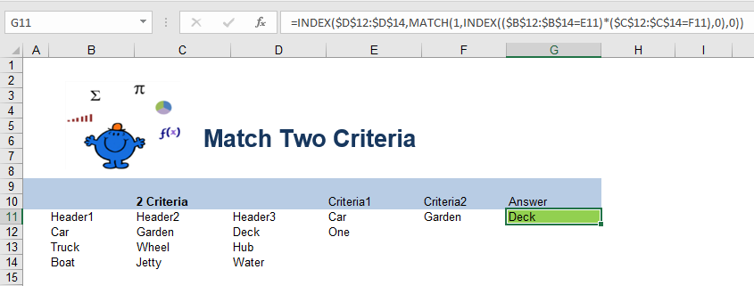
Using the above simple example we have 3 Excel columns, we want to match criteria in column 1 and column 2 to return the data in column 3.  In the above example we want to match;

Car and Garden to return Deck

The Excel formula to achieve this based on the above is as follows.

=INDEX($D$12:$D$14,MATCH(1,INDEX(($B$12:$B$14=E11)*($C$12:$C$14=F11),0),0))

Where Range D12:D14 contains the column information we want to return. Range B12:B14 contains the first criterion which is equal to E11 (Car). Range C12:C14 contains the final criterion which is equal to F11 (Garden).

Match 3 Criteria

This technique can be extended to include more criteria.  The following would be example of three criteria in an Excel formula.

=INDEX($E$12:$E$14,MATCH(1,INDEX(($B$12:$B$14=F11)*($C$12:$C$14=G11)*($D$12:$D$14=H11),0),0))

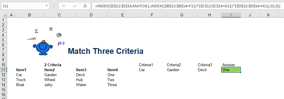
You don’t need to stop at 3 criteria either. The formula can go on and on. All you have to do is add an additonal multiplication * symbol a bracket then enter the range and criteria. There you go.

The attached Excel file contains both of the above examples.