
Updating Pivot Tables Automatically
Excel Pivot tables are fantastic for creating fast and accurate, sorted, summary information in Excel. To update a pivot table, traditionally you have to update the source data and either right click on the pivot table and click on the Refresh Button or Click on the Refresh button at the top of the screen;
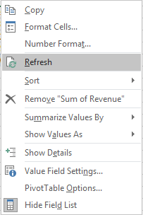
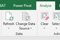
Either refresh by right clicking on the Pivot Table and the menu on the left will appear, click on refresh. Or you could click on the PivotTable Tools and click the refresh button.
Either option leaves you open to the possibility that the pivot table will not be updated as the user has to remember to update the pivot table whenever the source data has been updated.
Having an Excel pivot table update automatically is a valuable tool when dealing with data which changes on a regular basis. The idea is to have a dataset populated and have the pivot table update to reflect this change. There are a few ways you can do this. The first method I will describe is to create a Dynamic Named Range in Excel. Then in VBA add a Worksheet Activate Event which will Refresh the pivot table when you click on the worksheet.
Consider the following example data set. The data starts in Column A and always ends in Column E. I will call the dynamic range Source and the formula for the named range is;
=OFFSET(Data!$A$1,0,0,COUNTA(Data!$A$1:$A$20000),5)
The Column headers start in Row 1 of Column 1 (A1) I have used an upper bounds of the range of 20,000 rows. As I know my data will never go beyond this point. I have offset the columns by 5 which means the source data will be 5 columns wide. It will take the last used row in Column A and offset that by 5 Columns. Change to suit. If you don’t know how many columns are going to be in the pivot table use a dynamic formula like this.
=OFFSET(Data!$A$1,0,0,COUNTA(Data!$A:$A),COUNTA(Data!$1:$1))
If your data is based on a static range all you need to do now is change the source data to be equal to the dynamic range.
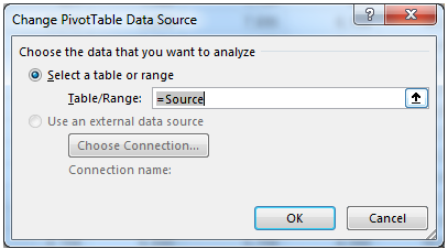
Now simply type in=Source
Note: Source needs to be the name of your dynamic named range.
The VBA Procedure
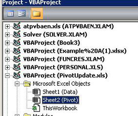
The following Excel VBA procedure needs to be placed in the Worksheet Object where the Pivot Table resides.
The Excel VBA code is as follows;
Private Sub Worksheet_Activate() 'Excel VBA to refresh a pivot table.
Dim pt As PivotTable
To test the above VBA coding go to the bottom of your dataset and put a new line of unique data. This is so you will be easily able to spot the update in your pivot table. As you click on the pivot table sheet you should see that unique piece of data added to the summary table. If you see that it works now go back and delete the line and when you click back into the pivot table sheet the data should be gone.
The same process can be achieved with VBA. Create a regular named Range called Source1 and follow the same steps to connect your pivot table up to the named range.
Now place the following VBA code into the Worksheet Object.
Private Sub Worksheet_Activate()' Excel VBA to update pivot table automatically.
Dim sh As Worksheet
Dim pt As PivotTable
Set sh = Sheet2
sh.Range("A10").CurrentRegion.Name="Source1"
End Sub
Notice how the Source1 named range is updated directly in VBA. The name for this pivot table range is Source1.
Filtered a Pivot Table by an External List
For long lists inside a pivot table it might be an idea to have data in a separate list and simply loop through that list. The Excel VBA to do so is as follows;
Sub FilterPiv() 'Excel VBA to filter the Pivot Table by a list outside the pivot Table.
Dim i As Integer
Application.ScreenUpdating= False
Dim pi As PivotItem
For Each pi In .PivotItems
For i=12 To Range("G" & Rows.Count).End(xlUp).Row
The following Excel file outlines the VBA procedures above.
