Cascading List with Formula

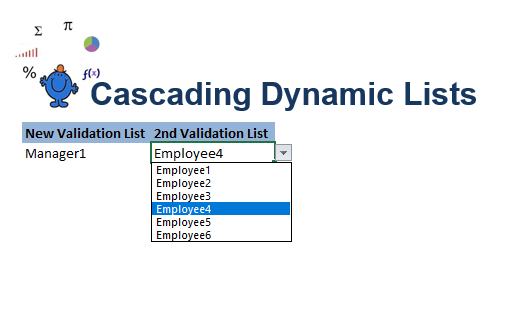
This article shows you how to set up a cascading drop down menu with formulas. Creating data validation lists which are linked to one another with Excel formula is a handy technique to know.  Cascading data validation lists are helpful when using categories and sub-categories which show the relationship between the category selected and its sub category.  So when you select a value from the first list, only the values related to that list are shown in the second list.  These type of set ups are relatively straight forward for a two validation list.  It becomes more complex for 3 or more.  The Excel VBA article Cascading Drop Downs in Excel might be of help as it takes the concept one step further.  I have seen this method achieved with named ranges and the Indirect function.  However, the following method will achieve the result with 5 named ranges and this will suffice no matter how long the first list is.  Here is a picture to show what a cascading drop down is made up of.

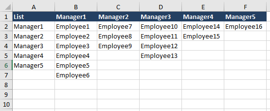
In Column A you have your list of Managers.  In Columns B to F you have those managers and the staff that work under them.  So from the following picture.

When you choose a manager on left in blue, only the managers displayed under their name are available in the data validation list.

To recreate the above 2 level dynamic drop down list with formula you will need the following formula.  The names at the top (Header for example) are the names I have given to each named range.

Header Excel formula:
=List!$A$1:INDEX(List!$1:$1,MATCH(REPT("z",255),List!$1:$1))

FirstRow Excel formula:
=ROW(List1!$A$1)

MatchColum Excel formula
=MATCH(Data!$A19,Header,0)

CurEntryCount Excel formula
=COUNTA(INDEX(List!$A:$GY,FirstRow+1,MatchColumn):INDEX(List!$A:$GY,65536,MatchColumn))

CurList Excel formula
=INDEX(List!$A:$GY,FirstRow+1,MatchColumn):INDEX(List!$A:$GY,FirstRow+CurrEntryCount,MatchColumn)

Attached is an Excel example of a cascading lists with formula.