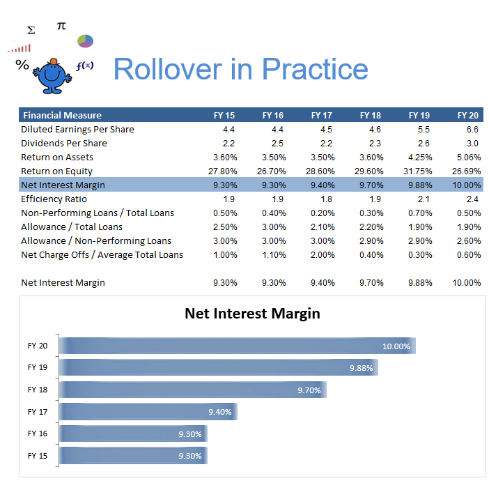
Chart Change Using Hyperlinks Part 2
The following article shows you how to create a cell rollover with the mouse using a hyperlink formula. In the first article on the mouse over or hyperlink method (Chart Hyperlinks) I showed how you can place your mouse over a cell to change a chart. I will take this concept one step further where you can use this method to highlight a line on a table with conditional formatting and change the focus of the table and the values on the chart. It is slightly different to the first article but the concept is the same.
Firstly we set up the custom function.
Incidentally the rng in the above is the range or cell which goes in the brackets of the hyperlink. The cell which will change will be cell B2.
Now we create a second list which is in a hidden or grouped column. Copy your list in the case above financial measures and paste them in an adjacent column. Now use the following formula in where you want the rollover event to happen. This is a 2003 formula as I will be saving the file in .xls format.
=IF(ISERROR(HYPERLINK(RollOver(P12),P12)),P12,HYPERLINK(RollOver(P12),P12))
If you are using a later version of Excel then the following will work too.
=IFERROR(HYPERLINK(RollOver(P12)),P12)
The formula is saying if the value in B2 which is our rng is the same as the value in P12 then this is the active row.
Now we just need a conditional formatting rule. Highlight your data table, Choose Conditional Formatting - New Rule - Use a formula to fetermine which cells to format.
Now put this rule;
=IF($C12=$B$2,1,0)
Change the style and interior colour. In the applies to section make sure it covers the full range.
That should do it. Now as you rollover each of your measures the whole line should change and bonus - the chart changes too!!! The following file shows workings.